Real-Time Kinematic (RTK)
Real-Time Kinematics (RTK): A High-Accuracy Positioning Technique with Reference-Station(-Networks)
RTK is a high-precision differential positioning technique using signals from Global Navigation Satellite Systems (GNSS). A centimetre-level positioning accuracy is enabled mainly by two aspects:
- The use of carrier phase measurements that are two to three orders of magnitude more precise than conventional pseudorange measurements.
- The correct resolution of the carrier phase integer ambiguities arising from the periodicity of the sinusoidal carrier signal.
RTK positioning uses the corrections from a reference station to reduce atmospheric (tropospheric and ionospheric) delays and satellite position, clock offset, phase and code bias errors and, thereby, to improve the positioning accuracy. Double differences are formed by (1) making differences between the measurements of the mobile receiver (rover) and the reference station, and (2) by further differencing the obtained single differences between any satellite and a common reference satellite. This double differencing reduces or eliminates the afore-mentioned errors.
1. Measurement model
RTK positioning typically uses three types of observables: pseudorange, carrier phase and Doppler measurements that are provided by the Delay Locked Loop (DLL), Phase Locked Loop (PLL) and Frequency Locked Loop (FLL) of a GNSS receiver. In this section, we present the measurement model for these types of observables.
1.1. Pseudorange Measurements
We start with the model for pseudorange measurements for satellite k observed by user u on frequency m given by:
\(
\newcommand{\R}[1]{{\mathrm{#1}}}
\begin{eqnarray*}
\rho_{u,m}^k &=& (\vec{e}_u^{\:k})^{\R{T}}\left(\vec{x}_u-\vec{x}^k\right) + c\left(\delta\tau_u-\delta\tau^k\right) + m_{\R{T}}(\theta_u^k)T_{\R{z},u} + q_{1m}^2I_u^k \\ && + b_{u,m} – b_m^k + \Delta\rho_{\R{MP},u,m}^k + \eta_{u,m}^k
\end{eqnarray*}
\)
with the following notations:
| Notation | Description |
| \( \vec{e}_u^{\:k} \) | Normalized line of sight vector from satellite to receiver |
| \( \vec{x}_u \) | Receiver position |
| \( \vec{x}^k \) | Satellite position |
| \( c \) | Speed of light |
| \( \delta\tau_u \) | Receiver clock offset |
| \( m_{\R{T}} \) | Tropospheric mapping function |
| \( \theta_u^k \) | Satellite elevation angle at receiver location |
| \( T_{\R{z},u} \) | Tropospheric zenith delay |
| \( q_{1m}^2 \) | Ratio of frequencies |
| \( I_u^k \) | Ionospheric slant delay on reference frequency (L1/ E1) |
| \( b_{u,m} \) | Receiver code bias |
| \( b_m^k \) | Satellite code bias |
| \( \Delta\rho_{\R{MP},u,m}^k \) | Pseudorange multipath error |
| \( \eta_{u,m}^k \) | Pseudorange measurement noise |
1.2. Carrier Phase Measurements
The carrier phase measurement is much less noisy but ambiguous (due to the periodicity of the sinusoidal carrier signal) and affected by other biases, i.e.
\(
\begin{eqnarray*}
\lambda_m\varphi_{u,m}^k
&=& (\vec{e}_u^{\:k})^{\R{T}}\left(\vec{x}_u-\vec{x}^k\right)
+ c\left(\delta\tau_u-\delta\tau^k\right)
+ m_{\R{T}}(\theta_u^k)T_{\R{z},u} – q_{1m}^2I_u^k \\
&& + \lambda_m N_{u,m}^k + \beta_{u,m} – \beta_m^k
+ \lambda_m\Delta\varphi_{\R{MP},u,m}^k + \varepsilon_{u,m}^k
\end{eqnarray*}
\)
with the following additional parameters:
| \( \lambda_m \) | Wavelength of carrier phase |
| \( N_{u,m}^k \) | Carrier phase integer ambiguity |
| \( \beta_{u,m} \) | Receiver phase bias |
| \( \beta_m^k \) | Satellite phase bias |
| \( \Delta\varphi_{\R{MP},u,m}^k \) | Carrier multipath error |
| \( \varepsilon_{u,m}^k \) | Carrier phase measurement noise |
1.3. Doppler Measurements
The Doppler measurement can be considered as a scaled version of the time-derivative of the carrier phase measurement. It is modelled as:
\(
\begin{eqnarray*}
f_{\R{D},u,m}^k
&=& -f_m/c\cdot\left((\vec{e}_u^{\:k})^{\R{T}}\left(\vec{v}_u-\vec{v}^k\right)
+ c\left(\delta\dot{\tau}_u-\delta\dot{\tau}^k\right)\right) \\
&& + \Delta f_{\R{D},\R{MP},u,m}^k + \eta_{f_{\R{D}},u,m}^k
\end{eqnarray*}
\)
with the following notations:
| \( f_m \) | Carrier frequency |
| \( \vec{v}_u \) | Receiver velocity |
| \( \vec{v}^k \) | Satellite velocity |
| \( \delta\dot{\tau}_u \) | Receiver clock drift |
| \( \delta\dot{\tau}^k \) | Satellite clock drift |
| \( \Delta f_{\R{D},\R{MP},u,m}^k \) | Doppler multipath error |
| \( \eta_{f_{\R{D}},u,m}^k \) | Doppler measurement noise |
1.4. Measurement Precorrections
The pseudorange and carrier phase measurements are then pre-corrected for the satellite position and clock offset estimates, i.e.
\(
\begin{eqnarray*}
\tilde{\rho}_{u,m}^k
&:=&
\rho_{u,m}^k + (\vec{e}_u^{\:k})^{\R{T}}\vec{x}^k + c\delta\tau^k \\
\lambda_m\tilde{\varphi}_{u,m}^k
&:=&
\lambda_m\varphi_{u,m}^k + (\vec{e}_u^{\:k})^{\R{T}}\vec{x}^k + c\delta\tau^k
\end{eqnarray*}
\)
Similarly, the Doppler measurements are pre-corrected for the satellite velocity and clock drift estimates, i.e.
\(
\tilde{f}_{\R{D},u,m}^k =
f_{\R{D},u,m}^k – f_m/c\cdot
\left(
(\vec{e}_u^{\:k})^{\R{T}}\vec{x}^k + c\delta\dot{\tau}^k
\right)
\)
1.5. Double Differences
The pre-corrected pseudorange and carrier phase measurements are double-differenced to eliminate the clock offsets and biases and to suppress the atmospheric delays:
\(
\begin{eqnarray*}
\tilde{\rho}_{ur,m}^{kl} &=&
\left(
\tilde{\rho}_{u,m}^k –
\tilde{\rho}_{u,m}^l
\right)
–
\left(
\tilde{\rho}_{r,m}^k –
\tilde{\rho}_{r,m}^l
\right) \\
&\approx&(\vec{e}_u^{\:kl})^{\R{T}}\vec{x}_{ur}
+ \Delta\rho_{\R{MP},ur,m}^{kl} + \eta_{ur,m}^{kl} \\\\
\lambda_m\tilde{\varphi}_{ur,m}^{kl} &=&
\left(
\lambda_m\tilde{\varphi}_{u,m}^k –
\lambda_m\tilde{\varphi}_{u,m}^l
\right)
–
\left(
\lambda_m\tilde{\varphi}_{r,m}^k –
\lambda_m\tilde{\varphi}_{r,m}^l
\right) \\
&\approx&(\vec{e}_u^{\:kl})^{\R{T}}\vec{x}_{ur} + \lambda_m N_{ur,m}^{kl}
+ \lambda_m\Delta\varphi_{\R{MP},ur,m}^{kl} + \varepsilon_{ur,m}^{kl}
\end{eqnarray*}
\)
which depend only on the relative position between the object receiver and the reference station, the double difference integer ambiguities, and the double difference multipath and noise.
The corrected Doppler measurements are also differenced between satellites to eliminate the receiver clock drift, i.e.
\(
\begin{eqnarray*}
\tilde{f}_{\R{D},u,m}^{kl}
&:=&
\tilde{f}_{\R{D},u,m}^k –
\tilde{f}_{\R{D},u,m}^l \\
&=&
– f_m/c\cdot
(\vec{e}_u^{\:kl})^{\R{T}}\vec{v}_u
+ \Delta f_{\R{D},\R{MP},u,m}^{kl} + \eta_{f_{\R{D}},u,m}^{kl}
\end{eqnarray*}
\)
2. Float RTK Solution with Kalman Filter:
The Kalman filter is a recursive least-squares estimator. It considers both the measurement models and a state space model. The Kalman filter minimizes the variance of the state estimates.
The differenced, pre-corrected pseudorange, carrier phase and Doppler measurements of one epoch (being indexed by n) are stacked in a single column vector:
\(
\begin{eqnarray*}
z_n &=&
\left(
\tilde{\rho}_{ur,1}^{1l},
\ldots,
\tilde{\rho}_{ur,1}^{Kl},
\ldots,
\tilde{\rho}_{ur,M}^{1l},
\ldots,
\tilde{\rho}_{ur,M}^{Kl},\right.\\
&&
\quad
\lambda_1\tilde{\varphi}_{ur,1}^{1l},
\ldots,
\lambda_1\tilde{\varphi}_{ur,1}^{Kl},
\ldots,
\lambda_M\tilde{\varphi}_{ur,M}^{1l},
\ldots,
\lambda_M\tilde{\varphi}_{ur,M}^{Kl},\\
&&
\left.
\quad
\tilde{f}_{\R{D},u,1}^{1l},
\ldots,
\tilde{f}_{\R{D},u,1}^{Kl},
\ldots,
\tilde{f}_{\R{D},u,M}^{1l},
\ldots,
\tilde{f}_{\R{D},u,M}^{Kl}
\right)^{\R{T}}
\end{eqnarray*}
\)
which is related to the unknown state vector at this epoch
\(
\begin{equation*}
x_n =
\left(
(\vec{x}_{ur,n})^{\R{T}},
(\vec{v}_{u,n})^{\R{T}},
N_{ur,1}^{1l},
\ldots,
N_{ur,1}^{Kl},
\ldots,
N_{ur,M}^{1l},
\ldots,
N_{ur,M}^{Kl}
\right)^{\R{T}}
\end{equation*}
\)
according to the previously introduced measurement models. This state vector can be related to the state vector of the previous epoch by a state space model:
\(
x_n = \Phi_n x_{n-1} + \eta_{x_n}
\)
with the following notations:
| \( \Phi_n \) | State transition matrix |
| \( \eta_{x_n} \) | Process noise |
The Kalman filter consists of alternating state predictions and state updates. The state prediction uses the state space model and is written as:
\(
\begin{eqnarray*}
\hat{x}_n^- &=& \Phi_n \hat{x}_{n-1}^+ \\
\Sigma_{\hat{x}_n^-} &=&
\Phi_n \Sigma_{\hat{x}_{n-1}^+} \Phi_n^{\R{T}} +
\Sigma_{x_n}
\end{eqnarray*}
\)
whereas the second row describes the error propagation in terms of the covariance matrix.
The state update first determines the innovation and subsequently uses it to correct the state prediction, i.e.
\(
\begin{eqnarray*}
\hat{x}_n^+ &=& \hat{x}_n^- +
K_n(z_n-H_n \hat{x}_n^-)\\
\Sigma_{\hat{x}_n^+} &=&
(1-K_nH_n)\Sigma_{\hat{x}_n^-}
\end{eqnarray*}
\)
with the Kalman gain
\(
K_n = \Sigma_{\hat{x}_n^-}H_n^{\R{T}}
\left(H_n\Sigma_{\hat{x}_n^-}H_n^{\R{T}}+\Sigma_{z_n}\right)^{-1}
\)
The position, velocity and ambiguity estimates are called the float RTK solution as the ambiguity estimates are real-valued.
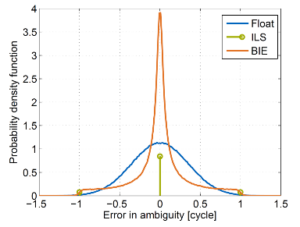
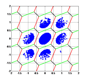
3. Integer Ambiguity Fixing – The Key to High Precision
The accuracy of the float RTK solution can be significantly improved by mapping the float ambiguities to integer ones. There exist a variety of integer ambiguity resolution techniques. The following table provides one overview of the most prominent integer resolution techniques and includes their definitions, advantages and disadvantages.
| Integer ambiguity resolution technique | Definition | Advantages | Disadvantages |
| Rounding | \begin{eqnarray*} \check{N}_{u,m,c}^k &=& \left[ \hat{N}_{u,m,c}^{k |1,\ldots,k-1} \right] \end{eqnarray*} |
|
|
| Bootstrapping | \begin{eqnarray*} \hat{N}_{u,m,c}^{k |1,\ldots,k-1} &=& \hat{N}_{u,m,c}^k – \sum_{j=1}^{k-1} \frac{\sigma_{\hat{N}_{u,m,c}^k\hat{N}_{u,m,c}^{j|1,\ldots,j-1}}}{\sigma_{\hat{N}_{u,m,c}^{j |1,\ldots,j-1}}^2} \\ && \cdot\left( \hat{N}_{u,m,c}^{j|1,\ldots,j-1}- \left[ \hat{N}_{u,m,c}^{j|1,\ldots,j-1} \right] \right) \end{eqnarray*} |
|
|
| Integer Least-Squares Estimation | \begin{eqnarray*} \check{N}_u &=& \R{arg}\min_{N_u} \|\hat{N}_u – N_u \|_{\Sigma_{\hat{N}_u}^{-1}}^2 \\ &=& Z^{-1}\left( \mathcal{S} \left(Z\hat{N}_u\right) \right) \end{eqnarray*} |
|
|
| Best-Integer Equivariant Estimation | \(
|
|
|
| Integer Aperture Estimation |
Ambiguity is mapped only to an integer if it lies in a pull-in region being given by:
\( |
|
|
| Best-Integer Equivariant Estimation | Integer Aperture Estimation |
 |
 |
4. Challenges of RTK and Potential Solutions
RTK positioning requires GNSS satellite visibility. Challenging environments with severe multipath and/ or limited satellite visibility might prevent an RTK integer ambiguity fixing. Moreover, measurement statistics might be inaccurate for highly-dynamic users in challenging environments.
The above challenges can be addressed by a sensor fusion with inertial measurements and wheel odometry. There exist different types of coupling, where as a tight coupling provides more accurate solutions than a loose coupling. For very challenging environments (e.g. tunnels, long sections in forests, etc.), an integration of visual sensors (camera or LiDAR) and a Simultaneous Localization and Mapping (SLAM) is recommended.
5. Applications of RTK Positioning
RTK positioning is very attractive for a wide range of applications including surveying, mapping, smart farming, robotics and automation, mining, the automotive, maritime, railway and aerospace (UAS) industries.
6. RTK Products of ANavS®
ANavS® is offering several products:
AI-ROX – The enhancement of the A-ROX system, with computer vision sensors including AI algorithmus.
A-ROX – GNSS-INS tightly coupled positioning system.
EmBox – Compact GNSS RTK and Heading Solution.
G-ROX – All-Frequency, all-Constellation RTK Reference Station.
Quick overview
Products
Equipped for every situation with the need of high-precise positioning & navigation:
AI-ROX, A-ROX, G-ROX, MSRTK, Snow Monitoring and M.2 SMART Card.
R&D Projects
Our R&D team is constantly working on researching, developing and implementing new technologies to master the challenges of tomorrow.
Publications
Our publications are varied, provide well-founded findings and present innovative solutions: Journal and Conference papers, Patents and Theses