Precise Point Positioning (PPP)
Precise Point Positioning (PPP): A High-Accuracy Positioning Technique without the need of additional Infrastructure
PPP is a high-precision absolute positioning technique using signals from Global Navigation Satellite Systems (GNSS). A decimetre-level positioning accuracy is enabled mainly by two aspects:
- The use of carrier phase measurements that are two to three orders of magnitude more precise than conventional pseudorange measurements.
- The use of orbital and clock corrections, phase and code biases, tropospheric and ionospheric corrections.
PPP positioning uses the corrections from service providers (e.g. IGS or Galileo High-Accuracy Service (HAS) by EUSPA) of reference station networks calculating the corrections and providing it by NTRIP-Casters to reduce atmospheric (tropospheric and ionospheric) delays and satellite position, clock offset, phase and code bias errors and, thereby, to improve the positioning accuracy. Single differences are formed by (1) making differences between the measurements of any satellite and a common reference satellite. This single differencing reduces or eliminates the afore-mentioned errors.
1. Joint Precise Point Positioning (PPP) and Attitude Determination
Converse to RTK positioning, the method of PPP does not require data of close-by reference receivers. Even though not as accurate as RTK, PPP offers a great accuracy in the magnitude of around 1-2 dm horizontally and approximately twice the value for the vertical positioning. The basis for this precise positioning is a consideration of several models, an estimation of more unknowns, and highly accurate satellite data. The latter needs to be provided by external correction services. However, in contrast to RTK, these corrections are globally valid and starting with the Galileo High Accuracy Service (HAS), they are potentially directly received from the satellites. Thus, no external communication link is necessary for highly precise positioning.
The pseudorange measurements and carrier phase measurements from a satellite received by a user on a frequency are given as follows.
1.1. Pseudorange Measurements
We start with the model for pseudorange measurements for satellite k observed by user u on frequency m given by:
\(
\newcommand{\R}[1]{{\mathrm{#1}}}
\begin{eqnarray*}
\rho_{u,m}^k &=& (\vec{e}_u^{\:k})^{\R{T}}\left(\vec{x}_u-\vec{x}^k\right) + c\left(\delta\tau_u-\delta\tau^k\right) + m_{\R{T}}(\theta_u^k)T_{\R{z},u} + q_{1m}^2I_u^k \\ && + b_{u,m} – b_m^k + \Delta\rho_{\R{MP},u,m}^k + \eta_{u,m}^k
\end{eqnarray*}
\)
with the following notations:
| Notation | Description |
| \( \vec{e}_u^{\:k} \) | Normalized line of sight vector from satellite to receiver |
| \( \vec{e}_u \) | Receiver position |
| \( \vec{x}^k \) | Satellite position |
| \( c \) | Speed of light |
| \( \delta\tau_u \) | Receiver clock offset |
| \( m_{\R{T}} \) | Tropospheric mapping function |
| \( \theta_u^k \) | Satellite elevation angle at receiver location |
| \( T_{\R{z},u} \) | Tropospheric zenith delay |
| \( q_{1m}^2 \) | Ratio of frequencies |
| \( I_u^k \) | Ionospheric slant delay on reference frequency (L1/ E1) |
| \( b_{u,m} \) | Receiver code bias |
| \( b_m^k \) | Satellite code bias |
| \( \Delta\rho_{\R{MP},u,m}^k \) | Pseudorange multipath error |
| \( eta_{u,m}^k \) | Pseudorange measurement noise |
1.2. Carrier Phase Measurements
The carrier phase measurement is much less noisy but ambiguous (due to the periodicity of the sinusoidal carrier signal) and affected by other biases, i.e.
\(
\begin{eqnarray*}
\lambda_m\varphi_{u,m}^k
&=& (\vec{e}_u^{\:k})^{\R{T}}\left(\vec{x}_u-\vec{x}^k\right)
+ c\left(\delta\tau_u-\delta\tau^k\right)
+ m_{\R{T}}(\theta_u^k)T_{\R{z},u} – q_{1m}^2I_u^k \\
&& + \lambda_m N_{u,m}^k + \beta_{u,m} – \beta_m^k
+ \lambda_m\Delta\varphi_{\R{MP},u,m}^k + \varepsilon_{u,m}^k
\end{eqnarray*}
\)
with the following additional parameters:
| \( \lambda_m \) | Wavelength of carrier phase |
| \( N_{u,m}^k \) | Carrier phase integer ambiguity |
| \( \beta_{u,m} \) | Receiver phase bias |
| \( \beta_m^k \) | Satellite phase bias |
| \( \Delta\varphi_{\R{MP},u,m}^k \) | Carrier multipath error |
| \( \varepsilon_{u,m}^k \) | Carrier phase measurement noise |
1.3. Doppler Measurements
The Doppler measurement can be considered as a scaled version of the time-derivative of the carrier phase measurement. It is modelled as:
\(
\begin{eqnarray*}
f_{\R{D},u,m}^k
&=& -f_m/c\cdot\left((\vec{e}_u^{\:k})^{\R{T}}\left(\vec{v}_u-\vec{v}^k\right)
+ c\left(\delta\dot{\tau}_u-\delta\dot{\tau}^k\right)\right) \\
&& + \Delta f_{\R{D},\R{MP},u,m}^k + \eta_{f_{\R{D}},u,m}^k
\end{eqnarray*}
\)
with the following notations:
| \( f_m \) | Carrier frequency |
| \( \vec{v}_u \) | Receiver velocity |
| \( \vec{v}^k \) | Satellite velocity |
| \( \delta\dot{\tau}_u \) | Receiver clock drift |
| \( \delta\dot{\tau}^k \) | Satellite clock drift |
| \( \Delta f_{\R{D},\R{MP},u,m}^k \) | Doppler multipath error |
| \( \eta_{f_{\R{D}},u,m}^k \) | Doppler measurement noise |
1.4. Measurement Precorrections
Utilising the concept of single differences, the terms which are common to a receiver are eliminated, i.e., the receiver clock offset as well as the receiver biases. While for RTK only the user position and the phase ambiguities need to be estimated, the atmospheric parameters for the zenith delay of the troposphere and for the ionospheric slant delays on the first frequency are also unknowns in the PPP algorithm. The ANavS positioning framework offers the possibility to also build the ionosphere-free combination of measurements to get rid of the slant delays as states of the estimating filter.
The complete procedure of all the modelling and estimation techniques can be found in the following figures.
2. Description of HAS PPP User Algorithm
This section includes a description of the proposed reference HAS PPP user algorithm. It uses a Kalman filter with an integrated partial or full integer ambiguity resolution, that processes satellite-satellite single differences of un-combined measurements as this approach is considered to be most attractive.
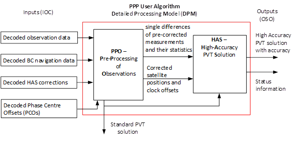
The following figure shows the two main blocks of the HAS PPP user algorithm that are relevant for the Detailed Processing Model (DPM) and their input and output interfaces. The first main block is the Pre-Processing of Observation, Navigation and Correction data (PPO), which includes e.g. the determination of the standard PVT solution and the forming of satellite-satellite single differences. The second main block includes the actual High Accuracy Service PVT solution (HAS) with a Kalman filter and integer ambiguity resolution.
2.1 Pre-Processing Software Module (PPO)
Pre-Processing steps (PPO) of HAS PPP User Algorithm:
- Determination of satellite positions, velocities, clock offsets and clock drifts
from broadcast ephemeris data - Determination of receiver position and clock offset with iterative least-squares (Standard PVT)
- Determination of absolute receiver velocity and clock drift with least-squares (Standard PVT)
- Determination of HAS-corrected satellite positions and clock offsets
- Checking of measurements for outliers
- Selection of a reference satellite for each constellation
- Determination of satellite-satellite single difference measurements
- 8a. Detection and correction of cycle slips
- 8b. Determination of measurement noise and process noise covariance matrices

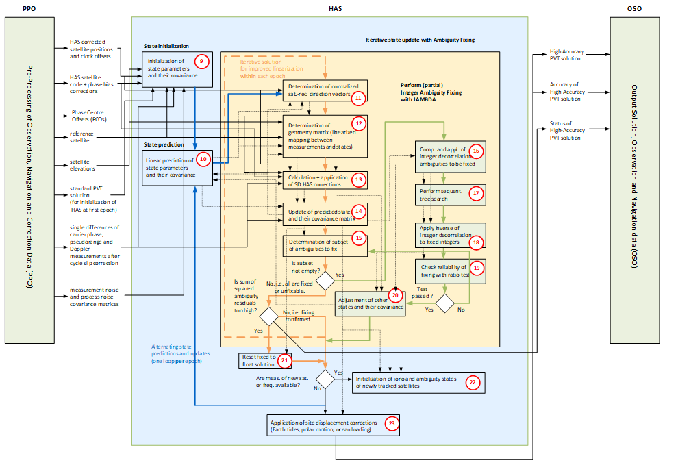
2.2 High Accuracy PPP Software Module (HAS)
Main processing steps (HAS) of HAS PPP User Algorithm:
- Initialization of state parameters:
Least-squares estimation of absolute receiver position, velocity, tropospheric zenith delay, ionospheric slant delays and float ambiguities using HAS-based pre-corrected SD measurements. - Linear prediction of state parameters
(position, velocity, tropospheric zenith delay, ionospheric slant delays and ambiguities)
Iterative state update (shown in orange)
- Determination of normalized satellite-receiver direction vectors
- Determination of geometry matrix (linearized mapping between states and measurements)
- Calculation and application of single difference HAS corrections
- Update of predicted states and their covariance matrix
with pre-processed measurements and their covariance matrix - Determination of subset of ambiguities to fix
Integer ambiguity fixing with LAMBDA (shown in green)
- Integer decorrelation of set of float ambiguities to be fixed
- Sequential tree search for determination of fixed integer vector candidates
- Application of inverse of integer decorrelation to fixed integer vector candidates
- Checking of reliability of best fixed integer candidate with ratio test
- Adjustment of all other states to exploit fixing of ambiguities
- Reset of fixed solution to float solution
- Initialization of ionospheric and ambiguity states for newly traced satellites
- Application of site-displacement corrections (Earth tides, polar motion and ocean loading)
3. Performance of PPP with HAS
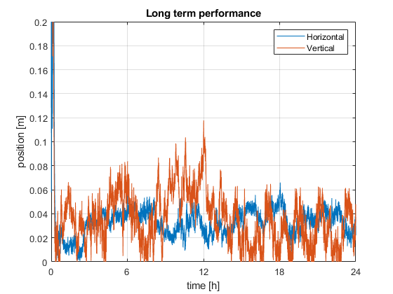
The following two figures show the accuracy performance and convergence behaviour of the PPP solution of ANavS as developed for the Galileo High Accuracy Service Reference User Algorithm and User Terminal (HAUT). The data set comprises a 24 hour period on the 13th of March 2022. The long term performance shows a great accuracy over a whole day. The convergence to a horizontal position offset of around 20 cm and a vertical of around 40 cm happen after approximately three minutes. A very accurate solution at centimetre level is available after 15-20 minutes.
The statistical performance for the complete data set is summarised by the 95-percentile of the horizontal and vertical deviation from the reference position, which is 4.8 cm and 7.4 cm, respectively.

Not visualised in the framework but a major part of it, is the combination of PPP with the determination of the attitude of the module. Therefore, double differences are computed to obtain baselines between receivers. Instead of estimating the baselines directly, the DD measurements and the geometry matrix serve as a basis for the estimation of a quaternion which represents the attitude without potential singularities. This results in an overall stacking of measurements from both PPP and GNSS attitude receivers in a single vector
4. Challenges of PPP and Potential Solutions
PPP positioning requires GNSS satellite visibility. Challenging environments with severe multipath and/ or limited satellite visibility might prevent an accurate PPP position convergency. Moreover, measurement statistics might be inaccurate for highly-dynamic users in challenging environments.
The above challenges can be addressed by a sensor fusion with inertial measurements and wheel odometry. There exist different types of coupling, where as a tight coupling provides more accurate solutions than a loose coupling. For very challenging environments (e.g. tunnels, long sections in forests, etc.), an integration of visual sensors (camera or LiDAR) and a Simultaneous Localization and Mapping (SLAM) is recommended.
5. Applications of PPP Positioning
PPP positioning is very attractive for a wide range of applications including surveying, mapping, smart farming, robotics and automation, mining, the automotive, maritime, railway and aerospace (UAS) industries.
6. PPP Products of ANavS®
ANavS® is offering several products for PPP positioning:
AI-ROX – The enhancement of the A-ROX system, with computer vision sensors including AI algorithmus.
A-ROX – GNSS-INS tightly coupled positioning system.
EmBox – Compact GNSS RTK and Heading Solution.
G-ROX – All-Frequency, all-Constellation RTK Reference Station.
Quick overview
Products
Equipped for every situation with the need of high-precise positioning & navigation:
AI-ROX, A-ROX, G-ROX, MSRTK, Snow Monitoring and M.2 SMART Card.
R&D Projects
Our R&D team is constantly working on researching, developing and implementing new technologies to master the challenges of tomorrow.
Publications
Our publications are varied, provide well-founded findings and present innovative solutions: Journal and Conference papers, Patents and Theses